Binomial Option Pricing Model
The binomial option pricing model values an option by working backward through discrete up-and-down price paths under no-arbitrage assumptions.
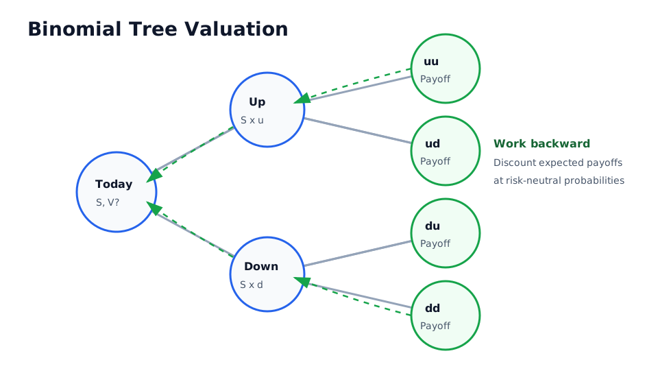
The binomial option pricing model values an option by building a tree of possible underlying prices and working backward from the option’s terminal payoffs. At each node, the model uses no-arbitrage logic to calculate continuation value and, for an American-style option, compares continuation with immediate exercise.
The result is a theoretical value under stated assumptions. It is not a guaranteed transaction price, trading profit, or forecast of the underlying asset.
Key Takeaways
- Each time step has an up branch and a down branch for the underlying price.
- No arbitrage requires the risk-free growth factor to lie between the down and up factors in the basic model.
- A derivative can be valued with a replicating portfolio or an equivalent risk-neutral expectation.
- Backward induction starts with expiration payoffs and values one earlier node at a time.
- American-style exercise is handled by choosing the greater of immediate exercise value and continuation value at each eligible node.
- Tree design, dividends, rates, volatility, time steps, exercise rules, and market frictions can materially change the output.
How a Binomial Tree Works
For current underlying price (S), one step produces:
and:
where (u) is the up factor and (d) is the down factor. A multi-period tree repeats these branches. In a recombining tree, an up move followed by a down move reaches the same price as a down move followed by an up move, reducing the number of distinct nodes.
For a simple non-dividend-paying one-period model with risk-free gross return (R), the no-arbitrage condition is:
If this condition fails, the assumed stock and risk-free asset prices permit a dominant trade within the simplified model. When it holds, the risk-neutral up probability is:
and (0<q_u<1). The risk-neutral weight is a pricing device implied by the model inputs, not necessarily the actual probability of an up move.
Worked Example: One-Period Call
Assume:
| Input | Value |
|---|---|
| Current stock price, (S_0) | $50 |
| Up factor, (u) | 1.20 |
| Down factor, (d) | 0.80 |
| One-period risk-free gross return, (R) | 1.05 |
| Call strike, (K) | $52 |
The stock can finish at $60 or $40. The call payoffs are:
The risk-neutral up probability is:
The call’s theoretical value is the discounted risk-neutral expected payoff:
The calculation does not say there is a 62.5% real-world chance that the stock will rise. It says that 0.625 is the pricing weight that makes the stock and risk-free asset consistent with no arbitrage in this two-state model.
Replication Cross-Check
The same price can be found by constructing a portfolio of stock and borrowing that matches the call’s payoff in both states.
The hedge ratio is:
Holding 0.40 share produces $24 in the up state and $16 in the down state. Borrowing $15.24 today creates a $16 repayment after one period at 5%. The terminal portfolio therefore pays:
| State | Stock holding | Loan repayment | Net payoff |
|---|---|---|---|
| Up | $24 | -$16 | $8 |
| Down | $16 | -$16 | $0 |
Its current cost is:
Because this portfolio reproduces the call payoff, a different call price would create an arbitrage in the frictionless model. Real implementation can differ because borrowing, shorting, rebalancing, transaction costs, liquidity, and discrete trading are not free.
Backward Induction
For a multi-period European option:
- Build the underlying-price tree.
- Calculate the option payoff at every expiration node.
- At each prior node, calculate the discounted risk-neutral expected value of its two successor nodes.
- Repeat until the initial node is reached.
At a node with next-step option values (V_u) and (V_d):
The model can accommodate node-specific rates, dividends, volatility, or branch factors, but those extensions must remain internally consistent.
American-Style Exercise
For an American Option, backward induction adds an exercise test:
This feature is important for contracts where early exercise can be valuable. The decision depends on option type, dividends or carry, rates, remaining time, and contract terms. A basic European Black-Scholes formula does not perform this node-by-node exercise comparison.
Choosing Tree Parameters
One common Cox-Ross-Rubinstein specification for time step (\Delta t), volatility (\sigma), continuously compounded rate (r), and continuous dividend yield (y) is:
This is one tree design, not the definition of every binomial model. Alternative trees match different moments, handle dividends differently, or improve convergence for particular payoffs.
Binomial vs. Black-Scholes
| Feature | Binomial model | Black-Scholes Model |
|---|---|---|
| Time | Discrete steps | Continuous-time closed form |
| Early exercise | Can be tested at each node | Basic formula assumes European exercise |
| Discrete dividends | Can be inserted at relevant nodes | Requires adjustment or another method |
| Contract flexibility | Useful for changing or path-dependent features | Best suited to standard European payoffs |
| Numerical behavior | Depends on step count and tree design | Immediate formula under its assumptions |
| Shared foundation | No-arbitrage replication | No-arbitrage replication |
As the number of properly specified steps increases, a binomial value may converge toward a continuous-time benchmark for a compatible payoff. More steps do not fix incorrect inputs or omitted contract features.
Common Mistakes
- Treating the risk-neutral probability as a forecast.
- Using (q_u) outside zero and one without diagnosing inconsistent inputs.
- Mixing annual rates, step rates, and compounding conventions.
- Omitting dividends, borrow costs, funding spreads, or settlement timing.
- Applying European backward induction to an American-style contract.
- Comparing trees with different volatility, calendar, or dividend conventions.
- Assuming more steps always produce monotonic or error-free convergence.
- Ignoring barrier monitoring, path dependence, dilution, or counterparty terms.
- Presenting theoretical value as an executable bid or offer.
How to Evaluate a Binomial Model
- Verify the option payoff, exercise style, expiration, strike, multiplier, and settlement terms.
- Match the underlying price, dividend assumptions, volatility, rate, and valuation timestamp.
- Document the tree type, step count, branch factors, and compounding convention.
- Confirm the no-arbitrage condition at each node.
- Test convergence across increasing step counts.
- Compare European-style results with an independent benchmark where appropriate.
- Review early-exercise boundaries and discrete-dividend treatment.
- Stress volatility, rates, dividends, and liquidity assumptions.
- Separate model value from executable market price and implementation cost.
Authoritative Sources
- Cox, Ross, and Rubinstein: Option Pricing, A Simplified Approach: university-hosted copy of the original discrete-time option-pricing paper.
- NYU Courant: Mathematics of Finance, Notes on Options: one-period replication, no-arbitrage conditions, risk-neutral weights, and multi-period trees.
- OCC: Characteristics and Risks of Standardized Options: contract and risk disclosures that remain relevant when a theoretical model is used.
Related Terms
- No Arbitrage: Price-consistency condition supporting replication-based valuation.
- Risk-Neutral Probabilities: Model-implied pricing weights used in the tree.
- Risk-Neutral Valuation: Broader framework for discounting expected payoffs under a pricing measure.
- Option Pricing Models: Comparison of theoretical option-valuation approaches.
- Model Risk: Risk that design, inputs, implementation, or use produces misleading output.
FAQs
Why does the binomial model work backward?
Can a binomial model value American options?
Does a risk-neutral probability predict the stock's direction?
This article provides general derivatives education. Options involve substantial risk, and model values do not guarantee executable prices, hedge performance, liquidity, or investment results.